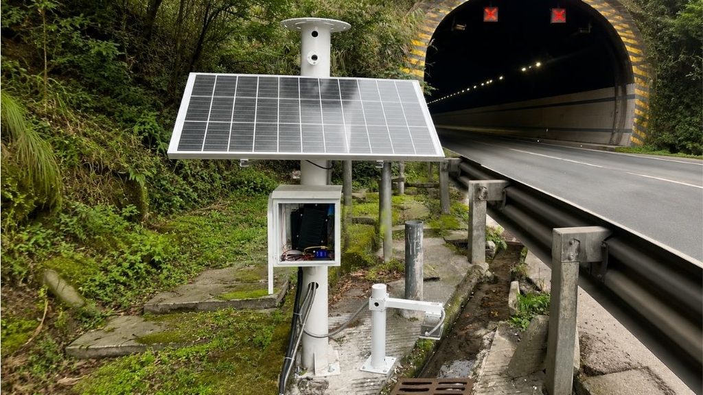
An open channel flow calculator is essential to measure water movement accurately in rivers and channels, plus irrigation systems where gravity drives flow with a free surface exposed to the atmosphere. Open channel flow serves as a key element in agriculture, flood control and ecosystems. Selecting the right open channel flow meter and applying open channel equations ensures precise measurements for water resource management. We’ll explore how radar and ultrasonic Doppler technologies work and get into different calculation methods for rectangular open channel flow and trapezoidal open channel flow calculator applications. This piece will help you choose the measurement system that fits your specific needs best.
Understanding Open Channel Flow and Flow Calculations
What is Open Channel Flow
Open channel flow occurs when liquid moves through a conduit with a free surface exposed to atmospheric pressure. Gravity serves as the driving force and pulls water from higher to lower elevations through channels like rivers, canals, and irrigation ditches. This is different from pipe flow, where pressure moves water through enclosed conduits. The free surface prevents pressure transmission from one end of the channel to another and makes gravity the sole mechanism for flow.
Flow classification depends on how depth and velocity change over time and distance. Steady flow means discharge at a point remains constant with time. Uniform flow requires no change in velocity magnitude or direction along a streamline so that flow depth stays constant. Non-uniform flow exhibits varying depth along the channel length. Most natural channels display non-uniform, unsteady, subcritical flow.
The Froude number determines flow behavior by comparing inertial forces to gravitational forces. Subcritical flow occurs when the Froude number falls below 1.0 and indicates flow depth exceeds critical depth. This tranquil, slow-moving water receives control from downstream direction. Supercritical flow, characterized by a Froude number above 1.0, exhibits rapid or shooting characteristics with depths less than critical depth. A Froude number equal to 1.0 indicates channel instability and should be avoided.
Parameters That Affect Flow Calculations
Cross-sectional area, wetted perimeter, and hydraulic radius are the geometric foundations for flow calculations. The cross-sectional area represents the water-carrying capacity perpendicular to flow direction. The wetted perimeter measures the total length where water contacts the channel boundary. Hydraulic radius, calculated as the ratio of cross-sectional area to wetted perimeter, indicates how a channel moves water.
Channel roughness affects flow velocity [substantially]. Manning’s roughness coefficient (n-values) for Texas streams and channels ranges from 0.012 to 0.200. Values outside this range are unrealistic. Determining the proper n-value is the most difficult and critical engineering judgment when using Manning’s equation. Smoother surfaces like grouted rip rap allow faster flow compared to natural channels with vegetation and debris.
Channel slope affects flow rate. Steeper slopes increase water velocity as gravitational force pulls water downward more [forcefully]. The slope, combined with roughness and hydraulic radius, determines the actual flow velocity through the channel. Manning’s equation incorporates these parameters to predict flow rates [accurately].
Common Open Channel Types: Rectangular and Trapezoidal
Rectangular channels feature flat bottoms with vertical sides. These channels offer simple analysis and construction with formwork, making them common in laboratory flumes and small drainage systems. Vertical sides create sharp corners that reduce hydraulic efficiency compared to sloped designs.
Trapezoidal channels provide superior stability and efficiency for most applications. The majority of open channels are trapezoidal with side slopes ranging from 1 to 3 (1 vertical to z horizontal) or flatter. Side slopes allow channels constructed in earth to maintain structural integrity while maximizing flow capacity. For a given cross-sectional area, trapezoidal channels minimize wetted perimeter better than rectangular designs and reduce friction losses.
The trapezoidal shape balances construction practicality with hydraulic performance. A regular hexagon filled halfway represents the most efficient trapezoidal channel. Semicircular channels need the least lining material but prove difficult to build. Trapezoidal channels emerged as the practical choice for irrigation canals and drainage systems, delivering efficiency without excessive construction complexity.
Open Channel Flow Equations and Calculation Methods
Manning’s Equation for Open Channel Flow
Manning’s equation estimates average velocity in open channels using an empirical formula: V = (k/n) × R^(2/3) × S^(1/2), where k equals 1.0 for SI units and 1.49 for English units. The discharge formula combines this with cross-sectional area as Q = A × V. Hydraulic radius (R) represents the ratio of flow area to wetted perimeter, while S indicates channel slope.
Accuracy under ideal conditions reaches 10-20%, but real-life measurements achieve 25-30% accuracy. Measurement conditions that vary can cause errors exceeding 50%. The roughness coefficient (n) introduces the greatest uncertainty. An error of ±20% in the n-value translates to ±20% error in calculated flow. Concrete channels have n-values that range from 0.010 for smooth surfaces to 0.027 for rough finishes. Natural streams exhibit higher values, from 0.030 for clean, straight channels to 0.150 for heavily vegetated reaches.
Velocity-Area Method
The velocity-area method calculates discharge by dividing the channel cross-section into subsections, measuring velocity and depth at each point, then summing partial discharges. The USGS recommends 25-30 subsections for typical measurements. No single subsection should carry more than 5-10% of total discharge.
Velocity measurements follow specific depth rules. A single reading at 0.6 times total depth from the surface provides adequate mean velocity in shallow streams (depth less than 0.75 meters). Deeper streams require two readings at 0.2 and 0.8 times depth, then averaged. Acoustic Doppler Current Profilers measure velocity profiles across entire cross-sections faster and prove valuable in deep or fast-flowing rivers where wading isn’t possible.
Weir and Flume Equations
The standard weir equation Q = C × L × H^(3/2) applies to most weir configurations. Sharp-crested weirs use coefficients of 3.33 (1.84 SI units), while Cipolletti weirs employ 3.367 (1.83 SI). Broad-crested weirs require lower coefficients around 3.09 (1.7 SI) due to different flow characteristics. Bridge deck overflow requires coefficients of 2.6, increasing to 3.0 for elevated roadway embankments.
Parshall flumes employ size-specific equations of the form Q = C × Ha^n. A 1-foot flume uses C=4.0 (imperial) with n=1.522, while larger 10-foot flumes use C=39.38 with n=1.6. Submergence limits vary by size: 50% for 1-3 inch flumes, 60% for 6-9 inch sizes, and 70% for 1-8 foot widths. Free-flow measurements achieve 3-5% accuracy when standard dimensions are maintained.
Continuity Equation (Q = A × V)
The continuity equation expresses conservation of mass in fluid mechanics. Discharge equals cross-sectional area multiplied by average velocity for steady flow of incompressible fluids. This relationship proves valid at all points along a channel and establishes that Q₁ = Q₂ or A₁V₁ = A₂V₂. Flow rate remains constant throughout the system, though area and velocity vary inversely at different sections.
Radar Flow Meters for Open Channel Measurement
How Radar Flow Meters Work
Radar flow meters transmit microwave signals toward the water surface at frequencies around 24 GHz. These signals strike moving water, and turbulence and ripples on the surface reflect the electromagnetic radiation back to the sensor. The returned signal exhibits a frequency shift due to the Doppler effect. This allows the device to calculate surface velocity. A separate radar component measures water level using time-of-flight principles. The system calculates distance based on signal travel time.
The measurement chain converts surface observations into total discharge. Surface velocity measurements get transformed into cross-sectional average velocity using site-specific coefficients, since surface speed exceeds mean velocity. The system determines wetted cross-sectional area by combining water level data with programmed channel geometry. Flow rate emerges from multiplying average velocity by cross-sectional area, plus a correction coefficient derived from actual field conditions.
FRM6002 Radar Flow Meter Technology
The FRM6002 operates with a speed range of 0.05 to 40 m/s and measurement accuracy of ±0.01 m/s. Its velocity measurement antenna employs a 10° × 27° beam angle. The ranging antenna uses a narrower 6° beam. Maximum ranging extends to 65 meters with accuracy of ±1 mm and a 20 cm blind spot. The device draws about 120 mA at 12V during normal operation.
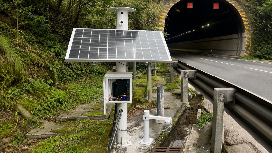
An IP68-rated aluminum alloy and PBT housing protects the unit. It functions in temperatures from -40°C to 85°C[204]. Communication occurs via RS485 Modbus protocol and Bluetooth 5.2. Measurement cycles complete in 0.5 to 2.5 seconds. Power supply accepts 7-28 VDC input and is compatible with solar installations for remote monitoring stations.
Built-in Channel Models: Rectangular, Trapezoidal, and Custom Shapes
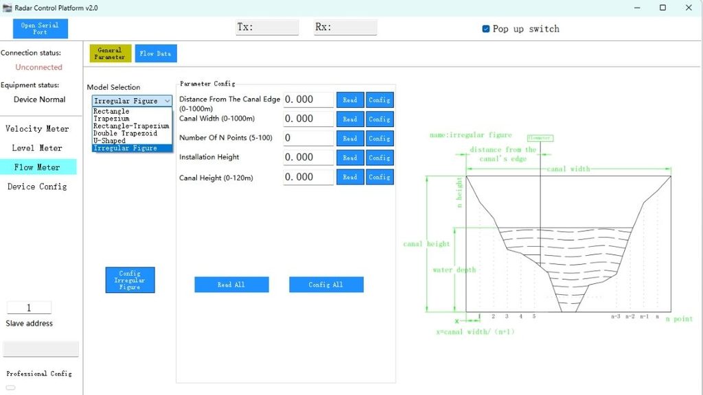
The FRM6002 has pre-programmed models for standard geometries: rectangular, trapezoidal, double trapezoidal, and U-shaped channels. The polygon model accepts custom coordinate points that describe the complete channel cross-section for irregular river sections. This flexibility eliminates the need for constructed weirs or flumes in natural waterways.
Operators input channel dimensions and select the appropriate geometric profile via RS485 software or Bluetooth during setup. The internal algorithm combines water level with stored geometry to calculate wetted area. It then applies velocity profile coefficients for accurate discharge determination.
Non-Contact Measurement Advantages
The sensor mounts above the water surface. This eliminates exposure to corrosive chemicals, abrasive sediment, and entangling debris. Maintenance demands drop substantially compared to submerged instruments. The radar continues functioning despite floating objects, aquatic vegetation, or high sediment loads that would compromise contact sensors.
Installation requires no channel modifications or flow interruption. Brackets attach to existing bridges, beams, or poles positioned over the waterway. This non-intrusive approach proves valuable in flood monitoring applications where rapid deployment matters and in remote locations where maintenance access is difficult.
Ultrasonic Doppler Flow Meters for Rivers and Channels
Doppler Effect Principles in Flow Measurement
Ultrasonic Doppler flow meters rely on frequency shifts that occur when sound waves reflect off moving particles in water. A transducer emits ultrasonic signals into the flow stream. Discontinuities such as suspended particles, air bubbles, or sediment reflect these waves back. The frequency of returned signals changes in proportion to the velocity of the reflecting particles, which move at the same speed as the surrounding water. This frequency shift, called the Doppler effect, is the foundation for calculating flow velocity. Doppler ultrasonic instruments require the presence of reflective particles in the fluid, unlike radar meters. This makes them unsuitable for clear water. So these meters excel in applications with wastewater, slurries and natural waterways where suspended matter occurs.
ADCP200 Acoustic Doppler Current Profiler
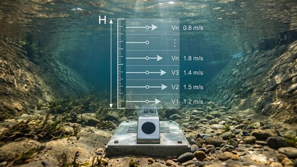
The ADCP200 operates at 2000 KHz frequency with a planar array single beam configuration. Its acoustic measurement range spans 0.06m to 25m with a blind zone of just 0.03m. The device measures velocity with ±0.5%±1.0mm/s accuracy and 0.001m/s resolution across a range of ±10m/s. What sets the ADCP200 apart is knowing how to divide the water column into up to 256 layers, with unit sizes adjustable from 0.25m to 25m. The instrument calculates discharge using the formula: Flow = Cross-sectional area × Average velocity, where cross-sectional area equals a1 + a2H + a3H² and average velocity derives from empirical coefficients combined with measured index velocity at different depths. Temperature sensing ranges from -25°C to 75°C with ±0.4°C accuracy.
SPDV200 Ultrasonic Doppler Transmitter
The SPDV200 emits ultrasonic waves obliquely upward into the fluid. These waves contact impurities moving with the water. Reflected signals produce a Doppler frequency shift (Δf) proportional to flow velocity. This transmitter measures velocities from ±0.03m/s to ±5m/s with ±1% flow rate accuracy. Water depth measurement extends from 0.02m to 3m (or 10m in custom configurations) with ±3cm accuracy and 1mm resolution. The device operates in temperatures from 0°C to 60°C and handles sand content up to 20g/L in pH ranges between 6 and 8. Applications include pipelines, channels and natural streams where direct contact measurement proves impractical.
Multi-Layer Velocity Profiling
ADCPs transmit acoustic pings that travel through the water column and measure current speed at multiple depths. The profiler captures velocity data across the entire depth profile with each ping series by measuring the time required for waves to bounce back and analyzing the Doppler shift. These instruments divide measurements into segments called range cells or bins. Each cell represents a specific depth layer. The first echoes return from the nearest range cell, while subsequent echoes arrive from deeper cells until signal strength dissipates. This technique measures water columns up to 1000m long and provides absolute water speed rather than relative movement between water masses.
Choosing the Right Open Channel Flow Meter
Channel Geometry and Size Requirements
Channel construction determines which measurement technology works best. Standard rectangular, trapezoid, or circular designs accommodate most open channel flow meters. Primary devices like flumes work by forcing flow through critical depth and require specific geometric constraints. People often overlook this point. Area-velocity meters, in contrast, adapt to existing channel shapes without structural modifications.
Flow Rate Range and Accuracy Needs
Your application’s permitting limits determine accuracy requirements. You need to figure out whether 3% accuracy proves necessary or 10% is enough. Ultrasonic level meters deliver flow rates with high accuracy at the time of use with well-maintained Parshall flumes. Applications where products get bought or sold based on meter readings just need absolute accuracy. Other uses prioritize repeatability.
Installation and Maintenance Considerations
Installation complexity varies between technologies by a lot. Older open channel flow metering products required precise installation. Slight missteps caused inaccurate readings or complete failure. Modern products simplified installation and programming, helping avoid common problems. Submerged sensors require frequent maintenance to clean in sanitary sewers. Non-contact measurements eliminate this burden but may face signal impedance from steam, condensate, or foam.
Environmental Factors: Sediment, Debris, and Water Quality
Sediment and debris affect measurement accuracy by a lot. Mag meters need particulates to get electrode readings. This makes them suitable where debris fills applications and ultrasonic meters struggle with impurities. Water conductivity matters for electromagnetic sensors and requires minimum 20 μS/cm.
Conclusion
Accurate flow measurement in open channels depends on selecting technology that matches your specific conditions. Radar meters like the FRM6002 excel with non-contact measurement and built-in channel models. Ultrasonic Doppler instruments such as the ADCP200 and SPDV200 provide detailed velocity profiling when particles exist in the water. Channel geometry, flow rate range, and environmental factors like sediment load determine which system delivers the best results. We recommend evaluating your accuracy requirements against installation complexity. The right open channel flow calculator transforms raw measurements into reliable data for water resource management and irrigation optimization. Choose your measurement system with care, and it will serve you for years.